Today I Read
Popularity versus similarity in growing networks
- Background
- Popularity and Similarity Together
- Variations and Emergent Models
- What else?
- References and Notes
Background
Why are we interested in networks? Because a enormous categories of phenomena can be modeled using networks. Internet, society, physics, biology, ecology, economy, even the evolution of the universe are essentially networks.
Concepts
- Degrees
Degrees. Source wikipedia.
Scaling in Networks
People have found a lot of scaling phenomena in networks.
- Internet links (directed links):
arXiv:cond-mat/0008465 for the scaling in internet links. What they find is that the distribution of degrees is power-law, i.e., $P\propto k^{-\gamma}$ with $\gamma\sim 2$. arXiv:cond-mat/0009090 provides a better explanation. The explanation is simply popular is more attractive.
- Barabasi et al found that in random networks, scaling appears also 1.
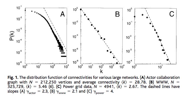
Scaling of connectivities. Barabasi (1999).
- And some theories like 2, etc.
Popularity
In the example of internet links, popular is attractive can be modeled by a dynamic generation of network following some rules.
- At each step we have $m$ links distributed.
-
The probability of attaching to some node with degree $k_i$ is
\[P_i \sim k_i + A\]where $A$ serves as a initial attractiveness since it tells us the probability of attachment when the degree $k_i=0$.
Dorogovtsev et al proved that this model gives us the final distribution of degrees
\[P \propto k^{-\gamma},\]where $\gamma=2 + A/m$ 3.
Similarity
The problem about popularity is that we are all aware that popularity is not the only factor.
Consider the following examples.
- You write a blog about neuroscience. In the past people usually put links on the blog, which is called blogroll or something. In the links, what you would include is something like facebook, google, maybe nature/science, and most likely some blogs or resources about neuroscience eventhough these websites may not be very popular. However, these links have similar contents as yours.
- We could also check the link you used in your articles and they are very likely to point to some websites that is also neuroscience.
In some cases similar is also important.
Popularity and Similarity Together
What we would expect is that larger popularity and small similarity (more similar) are the preferable connections. Thus competitions between the two determines the overall connection probability.
To combine the two factors, we use the metric $\mathrm{Popularity}\times \mathrm{Similarity}$. Even though there is a competition between popularity and similarity, small values of $\mathrm{Popularity}\times \mathrm{Similarity}$ are more preferable connections, which takes similarity more seriously.
A simple model to demonstrate this is to build a space of disc. The radius is time $t$, while angles are the measure of similarity. A smaller angler distance indicates a smaller similarity. Using this mapping, we are able to show the dynamics of networks, since we can tell the history of the nodes.
Mathematically speaking, the similarity is measured as
\[\begin{equation} \theta_{ij} = \lvert \theta_i - \theta_j \rvert. \end{equation}\]while time is the radius with $t=0$ at the center of the disc.
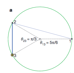
Disc of similarity. This figures shows the measure of similarity. 2 & 3 are more similar, given the fact that their angular distance $\lvert\theta_2-\theta_3\rvert$ is smaller that either $\theta_2-\theta_1$ or $\lvert\theta_3-\theta_1\rvert$. Papadopoulos et al (2012).
Now we are going to dynamically generate a network. The updating rules are listed bellow.
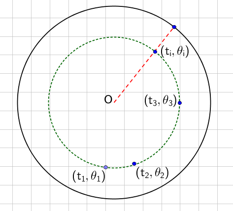
- We create a node at each time step and label them with numbers. For example, node 3 means it was created at time step 3. We denote the time of the $i$th node as $t_i$ and its angle on the disc as $\theta_i$.
- As the node $i$ is created at time $t_i$, it is connected to $m$ previous nodes.
- The node $i$ is connected to node $j$’s if $t_j\theta_{ij}$ are the smallest. In this measure $t_j$ is the popularity of node $j$ and $\theta_{ij}$ is the similarity of the two nodes.
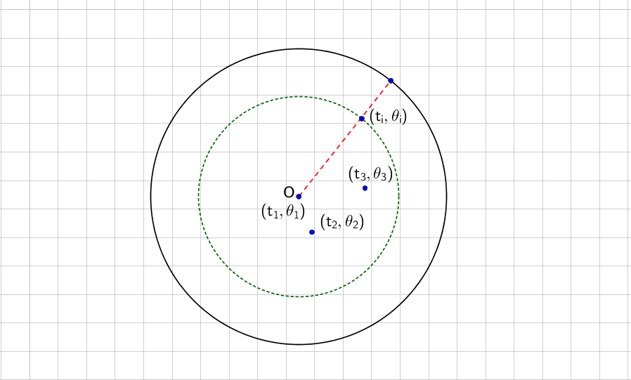
Illustration of the disc model. The radial coordinate measure the creation time of the node, while the angular distance measures the similarity.
The key transformation of this problem is to define a new radial coordinate system $r =\ln t$, so that the distance becomes log scale. Then we define the disc to be on a hyperbolic space so that the distance between any two points is calculated as 4
\[x_{ij} = r_i + r_j + \ln (\theta_{ij}/2) = \ln(t_i t_j \theta_{ij}/2).\]Minimizing $x_{ij}$ becomes equivalent to minimizing $t_j \theta_{ij}/2$ when dealing with the connectivity from a new born node $i$. The competition between popularity and similarity is simply the minimization of distance between two nodes on a hyperbolic plane.
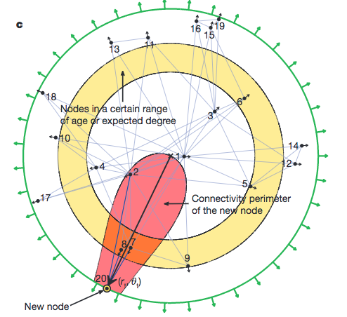
Illustration of the disc model. The radial coordinate measure the creation time of the node, while the angular distance measures the similarity. The shaded region is the a region enclosed by a equal distance line. Papadopoulos et al (2012).
Why is this definition of distance far superior than the previous measure of $\mathrm{Popularity}\times \mathrm{Similarity}$? Or why do I care? Because the universe/nature itself measures distance on hyperbolic space, i.e., Minkowski space. It also shows us the hint that by choosing a proper metric we might be able to define distance between any nodes in any systems. The only question becomes which geometry.
This result is astonishing also because a discrete system is most likely generated dynamically according to some laws. The method of mapping nodes to a hyperbolic space provides a convenient metric or distance for us to find out the closest nodes. In other words, a node always connect to it’s nearest neighbors if the metric/distance is well defined.
Variations and Emergent Models
- Popularity Fading
In many real networks, early nodes are more popular. However, popularity decreasing with time can also be modeled. The idea is simple. We allow the nodes to drift away from the center along its own radial direction according to the restraint
\[\begin{equation} r_{j}(t) = \beta r_j + (1-\beta) r_{i}, \end{equation}\]where $r_j$ is an old node and it drifts, $r_i$ is the node at current time. Why would we do this? As $\beta$ approaches 1, we fall back to the situation that the nodes are stationary and no drifting is allowed. On the other hand, $\beta$ approaches 0 means we have all the nodes drifting to the circle of current time.
Drift of nodes for $\beta=1$. All nodes are moving to a circle of current time.
The drifting effectively decrease the connectivity of the old nodes since they are drifting away from the center. Another view of this fading is that the connection probability power law index $\gamma$ is larger, i.e.,
\[\begin{equation} \gamma = 1 + 1/\beta. \end{equation}\]- Growth of Internet Autonomous System
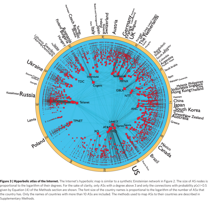
Internet AS on a hyperbolic disc. The radial coordinate is log of time, $r=\ln t$. Boguna et al (2010).
Boguna et al modeled the growth of internet AS using the popularity similarity method and it shows exactly the same statistical result as the actual internet AS data 5.
- Application to Cosmology
Krioukov et al came up with the idea that the whole universe can be mapped onto hyperbolic space and events are connected only to nearest neighbors. This in fact is already true in cosmology. Theories predicted that the matter density after inflation is power law, which can be explained by a dynamics generating of particle on a hyperbolic space. The authors created a map from the physical de Sitter space to hyperbolic space. Then the dynamic generation of the particles in the universe simple follows power law since the nodes generated this way has a power law distribution of degrees, i.e., a place that is dense initially is more likely to be dense after the inflation 6.
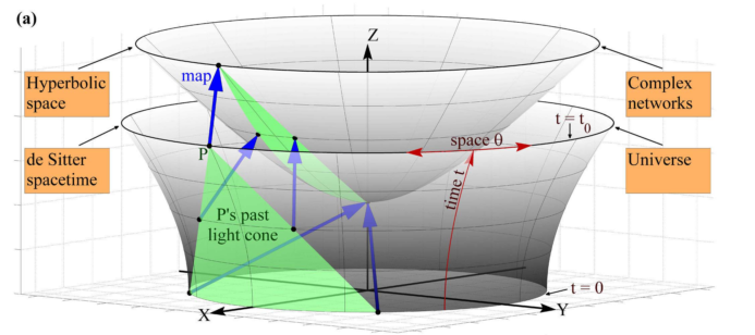
Map de Sitter space to hyperbolic space. Krioukov et al (2012).
What else?
- Such a network is very probabily optimized for information storage in the real world, because it stores information both in the global network and the local connections. An analysis of the snapshot of a network at a certain time shows a hierarchical structure which contains information about the past. The key feature of dynamics is explicitly stored in the network structure and easily extracted so that information storage is robust. Small world network is efficient for information storage and processing. It doesn’t explore all possible connection of the network while allowing information to be propagated through the whole network efficiently. The power law feature is a logarithmic compression of information about the the real world, which keeps the large scale information (low degree nodes) of an object but neglects details (large degree nodes).
- Does the brain follow the same law of dynamic generation of network? We know that the biological neural network is close to a small world network. Meanwhile, the popularityXsimilarity method models small world very well. As long as we find the proper metric/distance, we can confidently say that neural network always connect to the nearest neighbors.
- Artificial neural networks? We have to think about Boltzmann machine rather than the layerized artificial neural network. The question is, will a Boltzmann machine with network modeled by the method be very common if it actually solves a realistic problem?
References and Notes
-
Barabási, A.-L., & Albert, R. (1999). Emergence of Scaling in Random Networks. Science, 286(5439), 509–512. ↩︎
-
Krapivsky, P. L., Redner, S., & Leyvraz, F. (2000). Connectivity of growing random networks. Physical Review Letters, 85(21), 4629–4632. ↩︎
-
This express is specific for curvature $K=-4$. However, the final result of scaling doesn’t dependent on the curvature itself. ↩︎
-
Boguñá, M., Papadopoulos, F., & Krioukov, D. (2010). Sustaining the Internet with hyperbolic mapping. Nature Communications, 1(6), 1–8. ↩︎
-
Krioukov, D., Kitsak, M., Sinkovits, R. S., Rideout, D., Meyer, D., & Boguñá, M. (2012). Network Cosmology. Scientific Reports, 2, 793. ↩︎